Before beginning this final lab, please watch the short video below. Mila is going to provide a recap of the general concepts learned in the previous labs, explain briefly the climate models and the scenarios used in them, and describe some impacts of future climate change, before ending the video by reminding you of the three main questions you should be able to answer at the end of the lab.
This lab has 32 short-answer questions you will answer prior to the three big questions (i.e. , research questions) Mila has noted above.
Section 1
Here you are at the final lab of the climate-literacy labs, and at this juncture you are hopefully leaning towards the position that human activities have contributed to global environmental change. In fact, the information and evidence presented in the labs, beginning all the way back at Lab 2 (Stratospheric Ozone), show the profound impact that human activities, primarily through emissions of greenhouse gases into the atmosphere, have severely impacted atmospheric processes, energy budgets, etc. As you saw in Lab 8, the emissions of greenhouse gases from human activities has caused an imbalance in Earth’s energy budget and many changes in the atmosphere, hydrosphere, cryosphere, and biosphere have been observed over the past several decades. The figure below is the last figure you analyzed in Lab 8 and gives some examples of those changes.
This lab focuses on future climate change as projected through computer simulations. And based on what you saw we would expect to see continued glacier melting, reduction of permafrost, shrub increase in the Arctic, bleaching of corals, etc. if global warming does not stop. The modeling results in this lab show how temperature, precipitation, etc. are expected to change in the near-term (2016-2035) and in the long-term (2081-2100).
By the end of this lab, you should be able to answer the following research questions:
-
-
By the end of the century, how are temperatures across the globe projected to change under the scenarios with increasing CO2 concentrations?
-
How will continued increases in global temperature affect the global hydrologic cycle?
-
-
-
If global warming persists, how will the distribution of biomes at the end of the century differ from the current distribution?
-
__________________________________________________________________________________________
Entering with the right mindset
Throughout this lab you will be asked to answer some questions. Those questions will come in three different varieties:
![]() Fact based question →This will be a question with a rather clear-cut answer. That answer will be based on information (1) presented by your instructor, (2) found in background sections, or (3) determined by you from data, graphs, pictures, etc. There is more of an expectation of you providing a certain answer for a question of this type as compared to questions of the other types.
Fact based question →This will be a question with a rather clear-cut answer. That answer will be based on information (1) presented by your instructor, (2) found in background sections, or (3) determined by you from data, graphs, pictures, etc. There is more of an expectation of you providing a certain answer for a question of this type as compared to questions of the other types.
![]() Synthesis based question → This will be a question that will require you to pull together ideas from different places in order to give a complete answer. There is still an expectation that your answer will match up to a certain response, but you should feel comfortable in expressing your understanding of how these different ideas fit together.
Synthesis based question → This will be a question that will require you to pull together ideas from different places in order to give a complete answer. There is still an expectation that your answer will match up to a certain response, but you should feel comfortable in expressing your understanding of how these different ideas fit together.
![]() Hypothesis based question → This will be a question which will require you to stretch your mind little bit. A question like this will ask you to speculate about why something is the way it is, for instance. There is not one certain answer to a question of this type. This is a more open- ended question where we will be more interested in the ideas that you propose and the justification (‘I think this because . . .’) that you provide.
Hypothesis based question → This will be a question which will require you to stretch your mind little bit. A question like this will ask you to speculate about why something is the way it is, for instance. There is not one certain answer to a question of this type. This is a more open- ended question where we will be more interested in the ideas that you propose and the justification (‘I think this because . . .’) that you provide.
__________________________________________________________________________________________
Section 2: Radiative-Forcing Agents in Climate Models
Climate models (i.e., complex computer simulations) that serve as the primary tools available for investigating the response of the climate system to various forcings, for making climate predictions on seasonal to decadal time scales and for making projections of future climate over the coming century and beyond. It is extremely far beyond the scope of this lab to go into the details of the climate models from which the information in this lab is derived. But one important thing needs to be noted: all models are simplifications of reality and thus can substantial amounts of uncertainty attached to their predictions.
A major component of climate models is the inclusion of radiative-forcing agents, which enables the models to then simulate future climates. Therefore, climate models need information on how emissions and concentrations of things such as greenhouse gases aerosols will change in the future. Check out the table below showing the dozens of climate models and the forcing agents used in them.
![]() Q1: In addition to ozone, what four other greenhouse gases or groups of greenhouse gases are included in nearly all the climate models?
Q1: In addition to ozone, what four other greenhouse gases or groups of greenhouse gases are included in nearly all the climate models?
Climate models can’t model future climate without projections of future emissions of greenhouse gases and aerosols. Therefore, scientists and policy makers have created several different emissions scenarios for use in the IPCC’s Fifth Assessment Report. Watch the video below showing Dr. Sara Harris of the University of British Columbia (UBC) explain future emissions scenarios. This video is from Module 6.1 of UBC’s course Climate Literacy: Navigating Climate Change Conversations.
![]() Q2: With respect to the representative concentration pathways, what is the largest of the four hypothesized radiative forcings from pre-industrial times to 2100? The anthropogenic radiative forcing from 1750-2011 was 2.3 W m-2.
Q2: With respect to the representative concentration pathways, what is the largest of the four hypothesized radiative forcings from pre-industrial times to 2100? The anthropogenic radiative forcing from 1750-2011 was 2.3 W m-2.
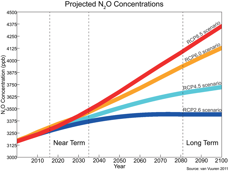
The three figures below expand on what you just saw in the video, which only showed projected CO2 emissions. The figures show projected CO2, CH4, and N2O emissions over the rest of the century. The scenario referred to as RCP3PD is named RCP2.6 hereafter in the lab.
![]() Q3: What two emissions scenarios most closely represent the current trend in CO2 emissions?
Q3: What two emissions scenarios most closely represent the current trend in CO2 emissions?
Below are the projected CO2, CH4, and N2O concentrations over the rest of the century. The atmospheric lifetimes of CO2 and N2O are approximately 100 years, while the lifetime of CH4 is roughly a decade. Near-term climate change is for the period 2016-2035, while long-term climate change is 2081-2100.
![]()
Q4: Why are CO2 concentrations increasing under the RCP4.5 scenario when emissions are decreasing?
__________________________________________________________________________________________
Section 3: Projected Temperature Changes
Combining the results from many climate models shows provides information like that provided in the figure below; it shows projected changes in the mean global temperature from 2005 to 2100. The values are differences from the mean global temperature from 1986-2005; therefore, the values are anomalies. The black line is an extrapolation of the linear trend in observed global temperature from 1979-2015.
![]() Q5: If we assume the current trend in temperatures will continue to occur until 2035, then how would you describe the projected changes from the four different scenarios in the near term (i.e., 2016-2035)?
Q5: If we assume the current trend in temperatures will continue to occur until 2035, then how would you describe the projected changes from the four different scenarios in the near term (i.e., 2016-2035)?
![]() Q6: Which scenario produces projections in the long term (i.e., 2081-2100) that most closely resembles the current trend in temperatures?
Q6: Which scenario produces projections in the long term (i.e., 2081-2100) that most closely resembles the current trend in temperatures?
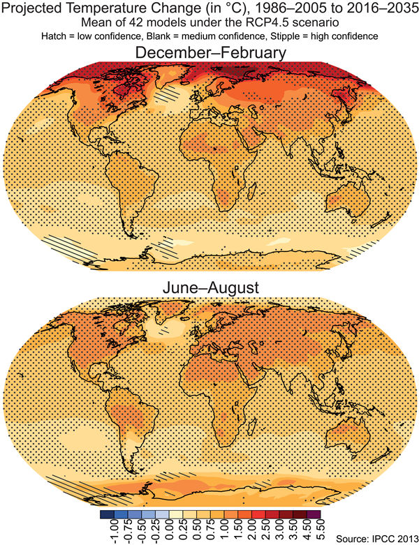
As you have seen the RCP6.0 and RCP8.5 scenarios matches an extrapolation of the current trend in CO2 emissions, while the RCP4.5 scenario in the long term most closely matches an extrapolation of the current trend in the mean global temperature. You also may have noticed that there was little disagreement among the scenarios with respect to projected emissions, concentrations, and temperatures in the near term. The RCP4.5 scenario is a “middle-ground” scenario, and the figures below show spatial variations in projected near-term temperatures under the RCP4.5 scenario. December-February and June-August are winter and summer, respectively, in the Northern Hemisphere.
![]() Q7: Why isn’t the Arctic region projected to warm more in the summer than in the winter? Think of a process that is consuming energy and not allowing that energy to become sensible heat.
Q7: Why isn’t the Arctic region projected to warm more in the summer than in the winter? Think of a process that is consuming energy and not allowing that energy to become sensible heat.
![]() Q8: If the figure above reflected results from using the RCP8.5 scenario in the climate models, then how would the temperature changes in the Arctic region differ from what you observed in the figure?
Q8: If the figure above reflected results from using the RCP8.5 scenario in the climate models, then how would the temperature changes in the Arctic region differ from what you observed in the figure?
__________________________________________________________________________________________
Section 4: Projected Changes in Evaporation and Atmospheric Moisture
The climate models also project changes in sea-surface temperature (SST), evaporation, and specific humidity, along with many other variables. The figures below show projected changes in SST, evaporation, and surface specific humidity in the near-term under the RCP4.5 scenario.
![]() Q9: What is the connection between SST and specific humidity? Think about the hydrologic cycle.
Q9: What is the connection between SST and specific humidity? Think about the hydrologic cycle.
![]() Q10: How might the projected increase in specific humidity affect the intensity of storm systems?
Q10: How might the projected increase in specific humidity affect the intensity of storm systems?
As you saw in the figure of projected mean global temperatures, there is a much larger temperature spread among the scenarios in the long term than in the near term. The figures below show projected changes in temperature from 1986-2005 to 2081-2100 under the four different scenarios.
![]() Q11: Why are land masses projected to warm more than the nearby oceans?
Q11: Why are land masses projected to warm more than the nearby oceans?
![]() Q12: What is the maximum amount of projected warming for any part of the Arctic? What is this warming in °F?
Q12: What is the maximum amount of projected warming for any part of the Arctic? What is this warming in °F?
__________________________________________________________________________________________
Section 5: Projected Changes in Storms, Precipitation, and Soil Moisture
Climate models also can make rough predictions in changes in the general locations of extratropical storms (i.e., storm systems poleward of the tropics). The figure below shows how the location of storm tracks in the winter season might change by the end of the century. Results using the RCP4.5 and RCP8.5 scenarios are shown for the Northern Hemisphere in the top two panels and for the Southern Hemisphere in the bottom two panels. The top two panels show the Northern Hemisphere and the bottom two panels show the Southern Hemisphere. It may seem somewhat counter-intuitive that places with projected decreases in extratropical storms are shown in shades of blue.
![]() Q13: How are the paths of extratropical storms expected to change?
Q13: How are the paths of extratropical storms expected to change?
![]() Q14: What extratropical regions not in Asia should experience much less rainfall in the future based on the projected changes in storm tracks?
Q14: What extratropical regions not in Asia should experience much less rainfall in the future based on the projected changes in storm tracks?
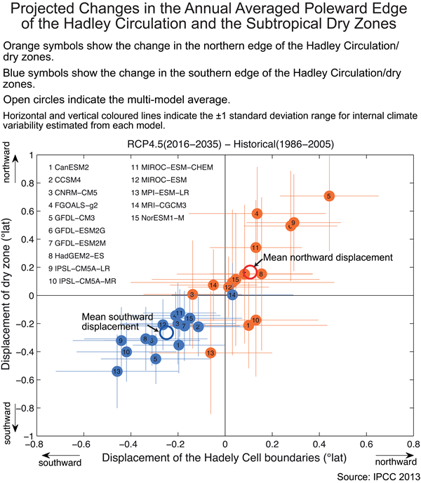
As you hopefully recall from Lab 3 (The Troposphere), a major feature of the tropics and subtropics is the Hadley Cell. This is the large-scale movement of air in the troposphere, with rising air at the ITCZ and sinking air outside the tropics in areas known as subtropical high-pressure cells. Humid air rises at the ITCZ, typically forms deep cumulonimbus clouds as it goes to the top of the troposphere, and then the air heads poleward and sinks in subtropical areas (i.e., subtropical highs). The figure on the right below shows projected changes by the end of the century in the locations of the northern and southern edges of the Hadley Cell under the RCP4.5 scenario.
![]() Q15: How is the width of the Hadley Cell expected to change?
Q15: How is the width of the Hadley Cell expected to change?
![]() Q16: What regions should experience much less rainfall in the future based on the projected changes in the Hadley Cell?
Q16: What regions should experience much less rainfall in the future based on the projected changes in the Hadley Cell?
Precipitation is an extremely difficult variable for climate models to predict, as illustrated by the hatching (i.e., low confidence in projections) in the figures below. The figure on the left shows projected precipitation changes in the near term under the RCP4.5 scenario. The figure on the right shows projected precipitation changes in the long term under the RCP8.5 scenario.
![]() Q17: How is Arctic precipitation projected to change?
Q17: How is Arctic precipitation projected to change?
![]() Q18: Why is precipitation over the Mediterranean region expected to decrease?
Q18: Why is precipitation over the Mediterranean region expected to decrease?
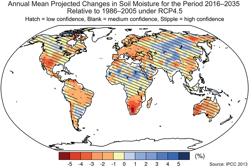
Climate models also can project future soil-moisture conditions. The amount of soil moisture is controlled by soil type, precipitation, and temperature. The figures from left to right show (1) projected near-term changes in soil moisture under the RCP4.5 scenario, (2) projected long-term changes in soil moisture under the RCP4.5 scenario, and (3) projected long-term changes in soil moisture under the four different scenarios.
![]() Q19: What specific changes in two climate variables are expected to lead to major decreases in soil moisture in southern Africa and the Mediterranean region?
Q19: What specific changes in two climate variables are expected to lead to major decreases in soil moisture in southern Africa and the Mediterranean region?
![]() Q20: How might agriculture in southern Europe change by the end of the century if conditions follow the RCP8.5 scenario?
Q20: How might agriculture in southern Europe change by the end of the century if conditions follow the RCP8.5 scenario?
The figure below summarizes the information in this section and the previous section by showing the general changes to the hydrologic cycle by the end of the century.
![]() Q21: How do the subtropics differ from high latitude areas with respect to changes in the hydrologic cycle?
Q21: How do the subtropics differ from high latitude areas with respect to changes in the hydrologic cycle?
__________________________________________________________________________________________
Section 6: Projected Changes to the Cryosphere
The graphic below shows observed changes to the cryosphere, and you examined this graphic at the end of the previous lab.
![]() Q22: Which of the changes noted in the figure above do you expect to continue throughout the rest of the century?
Q22: Which of the changes noted in the figure above do you expect to continue throughout the rest of the century?
Sea ice in the Northern Hemisphere reaches a maximum extent in February and a minimum extent in September. The image below shows projected changes in Northern Hemisphere sea ice over the rest of the century.
![]() Q23: Under the RCP4.5 scenario, how much is sea-ice extent in February expected to decrease from the 1986-2005 value by 2100? How much of a decrease is this in percent (i.e., divide the change by the 1986-2005 sea-ice extent value)?
Q23: Under the RCP4.5 scenario, how much is sea-ice extent in February expected to decrease from the 1986-2005 value by 2100? How much of a decrease is this in percent (i.e., divide the change by the 1986-2005 sea-ice extent value)?
![]() Q24: Under the RCP4.5 scenario, how much is sea-ice extent in September expected to decrease from the 1986-2005 value by 2100? How much of a decrease is this in percent (i.e., divide the change by the 1986-2005 sea-ice extent value)?
Q24: Under the RCP4.5 scenario, how much is sea-ice extent in September expected to decrease from the 1986-2005 value by 2100? How much of a decrease is this in percent (i.e., divide the change by the 1986-2005 sea-ice extent value)?
The image below shows where sea ice in the Northern Hemisphere is expected to decrease. Please be aware that not only is sea ice projected to decrease in extent but is also is projected to decrease in thickness, thereby continuing the current trends.
Notice that at the end of the century the Arctic Ocean is projected to be completely ice-free in late summer under the RCP8.5 scenario.
The extent and thickness of permafrost has been decreasing over the past several decades, and these changes are projected to continue. The figure below shows how the extent of permafrost, in millions of square kilometers, is projected to change by the end of the century under the four RCP scenarios.
![]() Q25: Based on the projected changes in permafrost area in the above figure, what climate type and what biome do you expect to shrink substantially in size by the end of the century?
Q25: Based on the projected changes in permafrost area in the above figure, what climate type and what biome do you expect to shrink substantially in size by the end of the century?
__________________________________________________________________________________________
Section 7: Projected Changes in Sea Level
Towards the end of the previous lab you learned that the observed rise in global mean sea level from 1993-2010 was 3.2 mm yr-1, and that thermal expansion was the largest contributor to the sea-level rise. If this rate of sea-level rise were to continue for 100 years the global mean sea level would rise by 0.32 meters.
Q26: What do you think is going to be the major contributor to sea level rise at the end of the century![]()
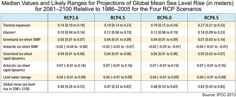
![]() Q27: What will continue to be the two major causes of sea level rise?
Q27: What will continue to be the two major causes of sea level rise?
The figure below shows the projected changes in sea level under the RCP4.5 scenario. And obviously coastal areas are the most impacted by sea-level changes. The Marshall Islands are one example of a region being impacted by past sea-level rise.
![]() Q28: How is rising sea level affecting the Marshall Islands?
Q28: How is rising sea level affecting the Marshall Islands?
![]() Q29: Based on the predictions in the above graphic, what is the prognosis for the Marshall Islands and other low-lying islands and coastal areas by the end of the century?
Q29: Based on the predictions in the above graphic, what is the prognosis for the Marshall Islands and other low-lying islands and coastal areas by the end of the century?
__________________________________________________________________________________________
Section 8: Projected Changes to Biomes
Biomes, which are formations of flora and fauna that have common characteristics, are controlled by the climate of a region. Throughout this lab you have seen that there might be dramatic changes in climate across the globe by the end of the century; therefore, there could be major shifts to biomes. You can observe possible changes in climate types from the present time to the end of the century be viewing the following Google Earth files: 1976-2000 and 2076-2100. These data were provided by the Institute of Veterinary Public Health of Vetmeduni Vienna. If you do not have access to Google Earth, then view the changing climate types here.
![]() Q30: What is the general movement of climate types (and thus biomes) in the middle and high latitudes of the Northern Hemisphere as you switch from 1976-2000 to 2076-2100?
Q30: What is the general movement of climate types (and thus biomes) in the middle and high latitudes of the Northern Hemisphere as you switch from 1976-2000 to 2076-2100?
![]() Q31: What biome would you expect to decrease the most in extent by the end of the century?
Q31: What biome would you expect to decrease the most in extent by the end of the century?
The figure below shows observed and projected changes associating with warming-induced shifting of the boreal forest and tundra biomes. Warming has caused the biomes to shift northwards, and the projected wrming is expected to continue the northward shift.
![]() Q32: What process resulting from the melting of tundra would lead to increased global warming?
Q32: What process resulting from the melting of tundra would lead to increased global warming?
__________________________________________________________________________________________
Section 9
Before the next lab, write for yourself a one-sentence response to each of the following big questions of this lab.
By the end of the century, how are temperatures across the globe projected to change under the scenarios with increasing CO2 concentrations
How will continued increases in global temperature affect the global hydrologic cycle?
If global warming persists, how will the distribution of biomes at the end of the century differ from the current distribution?


